Code
# load in the required modules

%matplotlib inline
import numpy as np
import matplotlib.pyplot as plt
import time
import gzip, os
from sklearn.neighbors import KDTree In this project, we will build a classifier that takes an image of a handwritten digit and recognizes the digit present in the image. Convolutional Neural Networks (CNNs) are usually preferred for such tasks because they are specifically designed to handle the spatial and hierarchical nature of image data, making them highly effective.
However, in this project, just for the sake of exploring a new technique, let’s explore a simple strategy, a non-learning method which is based on finding the nearest neighbor(s) (NN) to build the image classifier and see how it performs.
As brute force technique is used to find the nearest neighbor in our baseline NN classifier, let’s first work with a smaller dataset derived from our original dataset to reduce the computational time and make the algorithm work initially. Then, we will look at methods to improve the classification time that reduces the nearest neighbor search time.
Finally, note that this project is not about finding a good classifier for our dataset. Its rather about exploring some other technique and reasoning why it works and why it does not work.
# load in the required modules
%matplotlib inline
import numpy as np
import matplotlib.pyplot as plt
import time
import gzip, os
from sklearn.neighbors import KDTree We will use the MNIST dataset to create a subset of our original dataset. The full MNIST dataset contains training set of 60,000 images, and the test set of 10,000 images, where each image consists of a 28x28 grayscale image of a handwritten digit, along with corresponding labels (0 through 9) indicating the digit it represents.
But before creating a subset of our original dataset, let’s first explore our original dataset.
We first download a MNIST data file from Yann Le Cun’s website. Then, we define functions load_mnist_images and load_mnist_labels to convert the binary format to the numpy ndarray that we can work with.
# Reads the binary file and converts it into suitable numpy ndarray

def load_mnist_images(filename):
    with gzip.open(filename, 'rb') as f:
        data = np.frombuffer(f.read(), np.uint8, offset=16)
    data = data.reshape(-1,784)
    data = data.astype(np.float32)
    return data

def load_mnist_labels(filename):
    with gzip.open(filename, 'rb') as f:
        data = np.frombuffer(f.read(), np.uint8, offset=8)
return data# Load in the training set
original_train_data = load_mnist_images('train-images-idx3-ubyte.gz')
original_train_labels = load_mnist_labels('train-labels-idx1-ubyte.gz')
# Load in the testing set
original_test_data = load_mnist_images('t10k-images-idx3-ubyte.gz')
original_test_labels = load_mnist_labels('t10k-labels-idx1-ubyte.gz')# Print out the shape and no. of labels of the original dataset
print("Shape of the training dataset: ", np.shape(original_train_data))
print("Number of training labels: ", len(original_train_labels), end='\n\n')
print("Shape of the testing dataset: ", np.shape(original_test_data))
print("Number of testing labels: ", len(original_test_labels))Shape of the training dataset: (60000, 784)
Number of training labels: 60000
Shape of the testing dataset: (10000, 784)
Number of testing labels: 10000We can see that each data point, i.e., a handwritten digit image in the dataset, is composed of 784 pixels and is stored as a vector with 784 coordinates/dimensions, where each coordinate has a numeric value ranging from 0 to 255.
Let’s look at these numeric values by examining one of the images, say, the first image, in the dataset.
# print out the the first data point in training data

original_train_data[0]
array([ 0., 0., 0., 0., 0., 0., 0., 0., 0., 0., 0.,
0., 0., 0., 0., 0., 0., 0., 0., 0., 0., 0.,
0., 0., 0., 0., 0., 0., 0., 0., 0., 0., 0.,
0., 0., 0., 0., 0., 0., 0., 0., 0., 0., 0.,
0., 0., 0., 0., 0., 0., 0., 0., 0., 0., 0.,
0., 0., 0., 0., 0., 0., 0., 0., 0., 0., 0.,
0., 0., 0., 0., 0., 0., 0., 0., 0., 0., 0.,
0., 0., 0., 0., 0., 0., 0., 0., 0., 0., 0.,
0., 0., 0., 0., 0., 0., 0., 0., 0., 0., 0.,
0., 0., 0., 0., 0., 0., 0., 0., 0., 0., 0.,
0., 0., 0., 0., 0., 0., 0., 0., 0., 0., 0.,
0., 0., 0., 0., 0., 0., 0., 0., 0., 0., 0.,
0., 0., 0., 0., 0., 0., 0., 0., 0., 0., 0.,
0., 0., 0., 0., 0., 0., 0., 0., 0., 3., 18.,
18., 18., 126., 136., 175., 26., 166., 255., 247., 127., 0.,
0., 0., 0., 0., 0., 0., 0., 0., 0., 0., 0.,
30., 36., 94., 154., 170., 253., 253., 253., 253., 253., 225.,
172., 253., 242., 195., 64., 0., 0., 0., 0., 0., 0.,
0., 0., 0., 0., 0., 49., 238., 253., 253., 253., 253.,
253., 253., 253., 253., 251., 93., 82., 82., 56., 39., 0.,
0., 0., 0., 0., 0., 0., 0., 0., 0., 0., 0.,
18., 219., 253., 253., 253., 253., 253., 198., 182., 247., 241.,
0., 0., 0., 0., 0., 0., 0., 0., 0., 0., 0.,
0., 0., 0., 0., 0., 0., 0., 80., 156., 107., 253.,
253., 205., 11., 0., 43., 154., 0., 0., 0., 0., 0.,
0., 0., 0., 0., 0., 0., 0., 0., 0., 0., 0.,
0., 0., 0., 14., 1., 154., 253., 90., 0., 0., 0.,
0., 0., 0., 0., 0., 0., 0., 0., 0., 0., 0.,
0., 0., 0., 0., 0., 0., 0., 0., 0., 0., 0.,
139., 253., 190., 2., 0., 0., 0., 0., 0., 0., 0.,
0., 0., 0., 0., 0., 0., 0., 0., 0., 0., 0.,
0., 0., 0., 0., 0., 0., 11., 190., 253., 70., 0.,
0., 0., 0., 0., 0., 0., 0., 0., 0., 0., 0.,
0., 0., 0., 0., 0., 0., 0., 0., 0., 0., 0.,
0., 0., 35., 241., 225., 160., 108., 1., 0., 0., 0.,
0., 0., 0., 0., 0., 0., 0., 0., 0., 0., 0.,
0., 0., 0., 0., 0., 0., 0., 0., 0., 81., 240.,
253., 253., 119., 25., 0., 0., 0., 0., 0., 0., 0.,
0., 0., 0., 0., 0., 0., 0., 0., 0., 0., 0.,
0., 0., 0., 0., 0., 45., 186., 253., 253., 150., 27.,
0., 0., 0., 0., 0., 0., 0., 0., 0., 0., 0.,
0., 0., 0., 0., 0., 0., 0., 0., 0., 0., 0.,
0., 16., 93., 252., 253., 187., 0., 0., 0., 0., 0.,
0., 0., 0., 0., 0., 0., 0., 0., 0., 0., 0.,
0., 0., 0., 0., 0., 0., 0., 0., 0., 249., 253.,
249., 64., 0., 0., 0., 0., 0., 0., 0., 0., 0.,
0., 0., 0., 0., 0., 0., 0., 0., 0., 0., 0.,
0., 46., 130., 183., 253., 253., 207., 2., 0., 0., 0.,
0., 0., 0., 0., 0., 0., 0., 0., 0., 0., 0.,
0., 0., 0., 0., 0., 39., 148., 229., 253., 253., 253.,
250., 182., 0., 0., 0., 0., 0., 0., 0., 0., 0.,
0., 0., 0., 0., 0., 0., 0., 0., 0., 24., 114.,
221., 253., 253., 253., 253., 201., 78., 0., 0., 0., 0.,
0., 0., 0., 0., 0., 0., 0., 0., 0., 0., 0.,
0., 0., 23., 66., 213., 253., 253., 253., 253., 198., 81.,
2., 0., 0., 0., 0., 0., 0., 0., 0., 0., 0.,
0., 0., 0., 0., 0., 0., 18., 171., 219., 253., 253.,
253., 253., 195., 80., 9., 0., 0., 0., 0., 0., 0.,
0., 0., 0., 0., 0., 0., 0., 0., 0., 0., 55.,
172., 226., 253., 253., 253., 253., 244., 133., 11., 0., 0.,
0., 0., 0., 0., 0., 0., 0., 0., 0., 0., 0.,
0., 0., 0., 0., 0., 136., 253., 253., 253., 212., 135.,
132., 16., 0., 0., 0., 0., 0., 0., 0., 0., 0.,
0., 0., 0., 0., 0., 0., 0., 0., 0., 0., 0.,
0., 0., 0., 0., 0., 0., 0., 0., 0., 0., 0.,
0., 0., 0., 0., 0., 0., 0., 0., 0., 0., 0.,
0., 0., 0., 0., 0., 0., 0., 0., 0., 0., 0.,
0., 0., 0., 0., 0., 0., 0., 0., 0., 0., 0.,
0., 0., 0., 0., 0., 0., 0., 0., 0., 0., 0.,
0., 0., 0., 0., 0., 0., 0., 0., 0., 0., 0.,
0., 0., 0., 0., 0., 0., 0., 0., 0., 0., 0.,
0., 0., 0.], dtype=float32)# Compute the number of images of each digit in the training and test datasets
train_digits, train_counts = np.unique(original_train_labels, return_counts=True)
print("Training set distribution:")
print(dict(zip(train_digits, train_counts)), end='\n\n')
test_digits, test_counts = np.unique(original_test_labels, return_counts=True)
print("Test set distribution:")
print(dict(zip(test_digits, test_counts))) Training set distribution:
{0: 5923, 1: 6742, 2: 5958, 3: 6131, 4: 5842, 5: 5421, 6: 5918, 7: 6265, 8: 5851, 9: 5949}
Test set distribution:
{0: 980, 1: 1135, 2: 1032, 3: 1010, 4: 982, 5: 892, 6: 958, 7: 1028, 8: 974, 9: 1009}We can also see that our dataset is imbalanced. Now, let’s visualize some random images from the dataset.
# Reshape the data to be in the form of 28x28 images
X_train_images = original_train_data.reshape(-1, 28, 28)

# Select 16 random images to display
random_indices = np.random.choice(X_train_images.shape[0], 16, replace=False)
random_images = X_train_images[random_indices]
random_labels = original_train_labels[random_indices]  # Corresponding labels

fig, axes = plt.subplots(4, 4, figsize=(8, 8))

for i, ax in enumerate(axes.flat):
    # Plot each image on a subplot
    ax.imshow(random_images[i], cmap='gray')
    ax.set_title(f"Label: {random_labels[i]}")
    ax.axis('off')

plt.tight_layout()
plt.show()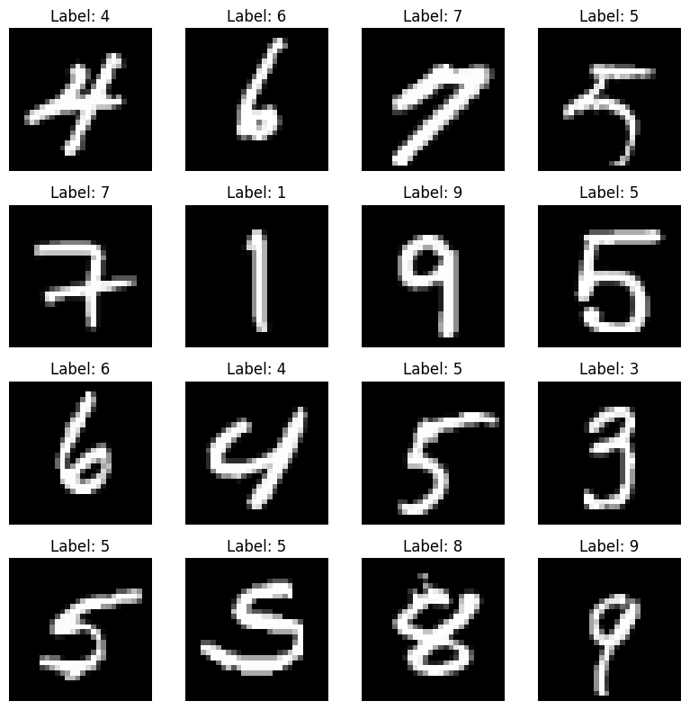
Now that we have explored our original dataset, let’s prepare a balanced dataset from it that contains 8000 samples for the training set and 2000 samples for the test set. Balanced dataset means samples are uniformly distributed across all labels (0 to 9) in both the sets. We define a function balance_dataset to carry out this task.
def balance_dataset(original_data, original_labels, samples_per_label):

    balanced_data = []
    balanced_labels = []

    # Iterate over each class label (here 0 to 9)
    for class_label in range(len(np.unique(original_labels))):

        # Find indices where the label equals the current class label
        indices = np.where(original_labels == class_label)[0]

        # Sample 'samples_per_class' indices uniformly from the current label
        sampled_indices = np.random.choice(indices, size=samples_per_label, replace=False)

        # Append the sampled data and labels to the balanced dataset
        balanced_data.append(original_data[sampled_indices])
        balanced_labels.append(original_labels[sampled_indices])

    # Concatenate the lists of arrays into single arrays
    balanced_data = np.concatenate(balanced_data, axis=0)
    balanced_labels = np.concatenate(balanced_labels, axis=0)

    # Shuffle the balanced dataset
    shuffle_indices = np.random.permutation(len(balanced_data))
    balanced_data = balanced_data[shuffle_indices]
    balanced_labels = balanced_labels[shuffle_indices]


return balanced_data, balanced_labels# preparing the balanced training and testing dataset
train_data, train_labels = balance_dataset(original_train_data, original_train_labels, 800)
test_data, test_labels = balance_dataset(original_test_data, original_test_labels, 200)Now, let’s also explore our balanced dataset.
# Compute the number of images of each digit in the training and test datasets

train_digits, train_counts = np.unique(train_labels, return_counts=True)
print("Training set distribution:")
print(dict(zip(train_digits, train_counts)), end='\n\n')

test_digits, test_counts = np.unique(test_labels, return_counts=True)
print("Test set distribution:")
print(dict(zip(test_digits, test_counts)), end='\n\n')


# Print out the shape and no. of labels of the balanced dataset

print("Shape of the training dataset: ", np.shape(train_data))
print("Number of training labels: ", len(train_labels), end='\n\n')

print("Shape of the testing dataset: ", np.shape(test_data))
print("Number of testing labels: ", len(test_labels))
Training set distribution:
{0: 800, 1: 800, 2: 800, 3: 800, 4: 800, 5: 800, 6: 800, 7: 800, 8: 800, 9: 800}
Test set distribution:
{0: 200, 1: 200, 2: 200, 3: 200, 4: 200, 5: 200, 6: 200, 7: 200, 8: 200, 9: 200}
Shape of the training dataset: (8000, 784)
Number of training labels: 8000
Shape of the testing dataset: (2000, 784)
Number of testing labels: 2000So in summary, we have prepared the following balanced dataset:
Now that we have our data ready, let’s first look at how we can compute the nearest neighbors.
To compute nearest neighbor in our dataset, we first need to be able to compute distances between data points (i.e., images in this case). For this, we will use the most common distance function Euclidean distance.
If x is the vector representing an image and y is the corresponding label, then:
Since we have 784-dimensional vectors to work with, the Euclidean distance between two 784-dimensional vectors, say \(x, z \in \mathbb{R}^{784}\), is:
\[\|x - z\| = \sqrt{\sum_{i=1}^{784} (x_i - z_i)^2}\]
where \(x_i\) and \(z_i\) represent the \(i^{th}\) coordinates of x and z, respectively.
For easier computation, we often omit the square root and simply compute Squared Euclidean distance:
\[\|x - z\|^2 = \sum_{i=1}^{784} (x_i - z_i)^2\]
The following squared_dist function computes the squared Euclidean distance between two vectors.
# Computes squared Euclidean distance between two vectors.

def squared_dist(x,z):
return np.sum(np.square(x-z))Let’s compute Euclidean distances of some random digits to see the squared_dist function in action before we use it in the NN classifier.
print('Examples:\n')

# Computing distances between random digits in our training set.

print(f"Distance from digit {train_labels[3]} to digit {train_labels[5]} in our training set: {squared_dist(train_data[4],train_data[5])}")

print(f"Distance from digit {train_labels[3]} to digit {train_labels[1]} in our training set: {squared_dist(train_data[4],train_data[1])}")

print(f"Distance from digit {train_labels[3]} to digit {train_labels[7]} in our training set: {squared_dist(train_data[4],train_data[7])}")
Examples:
Distance from digit 8 to digit 9 in our training set: 5624921.0
Distance from digit 8 to digit 4 in our training set: 5024177.0
Distance from digit 8 to digit 1 in our training set: 3521175.0Now that we have a distance function defined, we can turn to nearest neighbor classification.
In a nearest neighbor classification approach, for each test image in the test dataset, the classifier searches through the entire training set to find the nearest neighbor. This is done by computing the squared Euclidean distance between the feature vectors (in this case, the pixel values of the images) of the test image and all images in the training set. The image in the training set with the smallest Euclidean distance becomes the nearest neighbor to the test image, and the label of this nearest neighbor is assigned to the test image. This process is repeated for each test image, resulting in a classification for the entire test dataset based on the labels of their nearest neighbors in the training set.
we define the function NN_classifier() to find the nearest neighbour image for a given image x, i.e., the image that has least squared Euclidean distance, and then returns its label. The returned label is what the given image x could represent.
# Takes a vector x and returns the class of its nearest neighbor in train_data

def NN_classifier(x):


    # Compute distances between given image x and every image in train_data
    distances = [squared_dist(x, train_data[i]) for i in range(len(train_labels))]

    # Get the index of the image that resulted in smallest distance
    index = np.argmin(distances)

return train_labels[index]Let’s apply our nearest neighbor classifier to the full test dataset.
# Predict on each test data point and time it!

t_before = time.time()
test_predictions = [NN_classifier(test_data[i]) for i in range(len(test_labels))]
t_after = time.time()Since the nearest neighbor classifier goes through the entire training set of 8000 images, searching for the nearest neighbor image for every single test image in the dataset of 2000 images, we should not expect testing to be very fast.
# Compute the classification time of NN classifier

print(f"Classification time of NN classifier: {round(t_after - t_before, 2)} sec")
Classification time of NN classifier: 57.33 sec# Compute the error rate
err_positions = np.not_equal(test_predictions, test_labels)
error = float(np.sum(err_positions))/len(test_labels)
print(f"Error rate of nearest neighbor classifier: {round(error * 100, 2)}%")Error rate of nearest neighbor classifier: 5.45%The error rate of the NN classifier is 5.45%.
This means that out of the 2000 points, NN misclassifies around 109 of them, which is not too bad for such a simple method.
We have seen that our baseline model performs well and the brute-force search technique for the nearest neighbor is quite effective, but this method can be computationally expensive, especially with large datasets. If there are \(N\) training points in \(\mathbb{R}^d\), this approach scales as \(O(N d)\) time. That means the brute-force approach quickly becomes infeasible as the number of training points 𝑁 grows.
There are algorithms such as locality sensitive hashing, ball trees, k-d trees to optimize the nearest neighbor search by creating data structures on our data. In this project, we will explore k-d tree algorithm.
A k-d tree (k-dimensional tree) is a data structure used to organize points in a k-dimensional space. First, the k-d tree is built by recursively partitioning the data into two halves along one of the k dimensions. Next, during a nearest neighbor search, the algorithm uses the triangle inequality to determine whether it can prune certain branches of the tree (i.e., avoid searching certain subspaces). This allows the k-d tree to avoid unnecessary calculations, improving search efficiency thereby decreasing the classification time.
Here, we will use scikit-learn library to implement our k-d tree.
## Build nearest neighbor structure on training data

t_before = time.time()
kd_tree = KDTree(train_data)
t_after = time.time()

## Compute training time
t_training = t_after - t_before
print(f"Time taken to build the data structure: {round(t_training, 2)} sec")

## Get nearest neighbor predictions on testing data
t_before = time.time()
test_neighbors = np.squeeze(kd_tree.query(test_data, k=1, return_distance=False))
kd_tree_predictions = train_labels[test_neighbors]
t_after = time.time()

## Compute testing time
t_testing = t_after - t_before
print(f"Time taken to classify test set: {round(t_testing, 2)} sec", end = '\n\n')

## total classification time

print(f"Overall classification time of k-d tree algorithm: {round(t_training + t_testing, 2)} sec")
Time taken to build the data structure: 0.58 sec
Time taken to classify test set: 10.27 sec
Overall classification time of k-d tree algorithm: 10.85 secSo, the k-d tree has drastically reduced our classification time. It took just 10.27 seconds to classify the entire test set while taking only around 0.5 second to build the tree data structure. Therefore, the overall classification time is approximately 11 seconds.
Remember, the k-d tree algorithm only speeds up the nearest neighbor search; it does not affect the prediction process itself. The predictions of our baseline NN classifier will be the same as those of the k-d tree NN classifier. Let’s test this.
## Verify that the both predictions of baseline NN and k-d tree NN are the same

print("Does k-d tree produce same predictions as NN classifier? ", np.array_equal(test_predictions, kd_tree_predictions))
Does k-d tree produce same predictions as NN classifier? TrueNow let’s also look at how our k-d tree algorithm works on the original dataset i.e. dataset with 60,000 training images and 10,000 testing images.
t_before = time.time()
kd_tree = KDTree(original_train_data)
t_after = time.time()

## Compute training time
t_training = t_after - t_before
print(f"Time to build data structure: {round(t_training, 2)} sec")

## Get nearest neighbor predictions on testing data
t_before = time.time()
test_neighbors = np.squeeze(kd_tree.query(original_test_data, k=1, return_distance=False))
kd_tree_predictions = original_train_labels[test_neighbors]
t_after = time.time()

## Compute testing time
t_testing = t_after - t_before
print(f"Time to classify test set: {round(t_testing, 2)} sec", end = '\n\n')

## total classification time

print(f"Overall classification time of k-d tree algorithm: {round(t_training+t_testing, 2)} sec")
---------------------------------------------------------------------------
KeyboardInterrupt Traceback (most recent call last)
KeyboardInterrupt: The above code is taking forever so i have terminated it.
Although, k-d tree nearest neighbor worked well for smaller dataset it completely failed when the dataset grew bigger.
This could be due to the following reasons:
When we are working with smaller dataset i.e with only 8,000 training images, the tree structure built is relatively shallow and the number of points to compare during a nearest neighbor search is much smaller. This makes the algorithm’s computational load manageable. Whereas with the full dataset, the depth of the k-d tree increases which leads to more nodes. This results in an drastic increase in the time complexity of searches as the search frequently requires backtracking to different nodes and exploring other branches of the tree to find the nearest neighbor.
With more data points, the k-d tree requires more memory to store the nodes, which can lead to significant overhead. This increased memory usage can cause slower performance, it must be also noted that we are running the model on a 1.70 GHz Intel Core i7 (16GB RAM) laptop, which has limited computing power.
From the above observations, we can conclude that k-d trees can only be useful for specific tasks, especially in small or moderately-sized datasets or when a very simple model is sufficient.
Another thing to be noted here is the accuracy of k-d tree nearest neighbor or baseline NN depends on the quality of the data and the distance metric used. Here we used Euclidean distance which is affected by deformations in the image. But since our quality of the data is good, we did not face any such issues.
So in all practical cases especially when dealing with large, high-dimensional image datasets, more efficient methods like Convolutional Neural Networks (CNNs) are typically used as they are designed to handle high-dimensional data like images and generalize better because they learn from the data, rather than just memorizing it.